ENGR 362 Digital Signal Processing Project

In the ENGR 362 Digital Signal Processing project, we were presented a final project were students were to design a digital guitar compression pedal.

This project involved designing and implementing the digital signal processing (DSP) filters using MATLAB. An audio recording of a guitar playing a D Major chord was provided. The main notes are located at the frequencies of 146.83 Hz (D3), 220.00 Hz (A3), 293.66 Hz (D4), and 369.99 Hz (F#4).

Project Objectives

• Analyze: Plot and analyze the original audio in both time and frequency domains.
• Isolate: Design a parallel filter bank with four bandpass filters to isolate each individual note.
• Measure: Record the amplitudes of the filtered signals to balance them during recombination.
• Compress/Equalize: Equalize the amplitudes of the four frequencies to within 10% of each other, then recombine and analyze the final output.

Frequency Detection

The frequency detection was done by using MATLABs internal function findpeaks(). However, this function provided too much information, including smallpeaks that were beside larger peaks. In order to get the larger more prominent peaks, aloop was used to find peaks within 1% of another and remove the peak with a loweramplitude. The output was then truncated to provide only the 4 most prominent peaks.The number of peaks and percentage of which peaks are close can be adjustedthrough parameters.

Filter Design

The filters used were a 7th order Chebyshev low, and high pass filter each with the passband ripple being set to 0.5. Both filters were given a center frequency ± a percentage of width, with the low pass center frequency being set a fraction above the peak frequency, and the high pass having a center frequency a fraction below. During trials, compression within spec worked with a percentage between 1% and 8.875%.

To achieve the desired filter characteristics, the program was repeatedly run with various parameters adjusted each time. The parameters available were the order of the filter, the percentage above and below the center frequency that the low and high pass cutoff frequency was set to, and the passband ripple.

The passband ripple was not adjusted much, it was set to 0.5 to start. Adjusting the filters order adjusts the cutoff slope, and so a sharp slope was desired, therefore a 7th order filter was ideal. Having too low an order filter would increase the error between the peaks in the processed signal, making it not meet the 10% specification. The filter order could be increased given a larger width percentage, it entirely depends on how the user wants the processed signal to sound.

The width percentage was set to 8.875%, which resulted in a peak deviation of approximately 10%, therefore, the width percentage can be anywhere between 0% and 8.875% with the given audio file. To allow for some error, the width percentage was set to 5%, which resulted in a peak deviation of 3.75%.

The following figures show the filter's frequency response and each filtered signal in the time domain.

First is the frequency response of 7th order Chebyshev filters at peak frequencies with cutoff frequency widths being ±5% the peak frequency.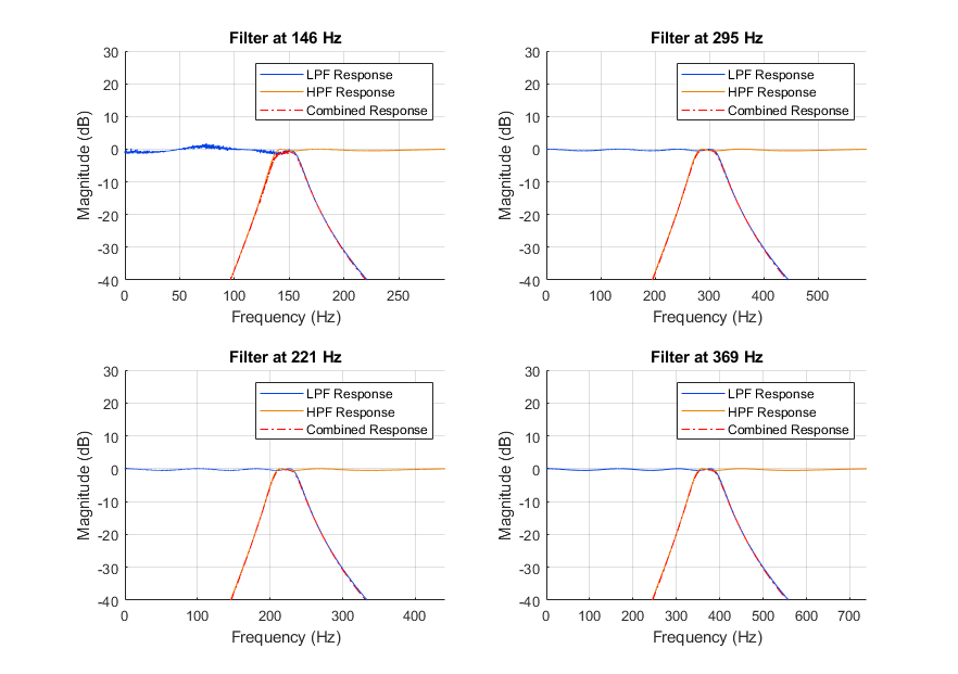

Next are the resulting peaks of each filtered signal at their respective frequencies.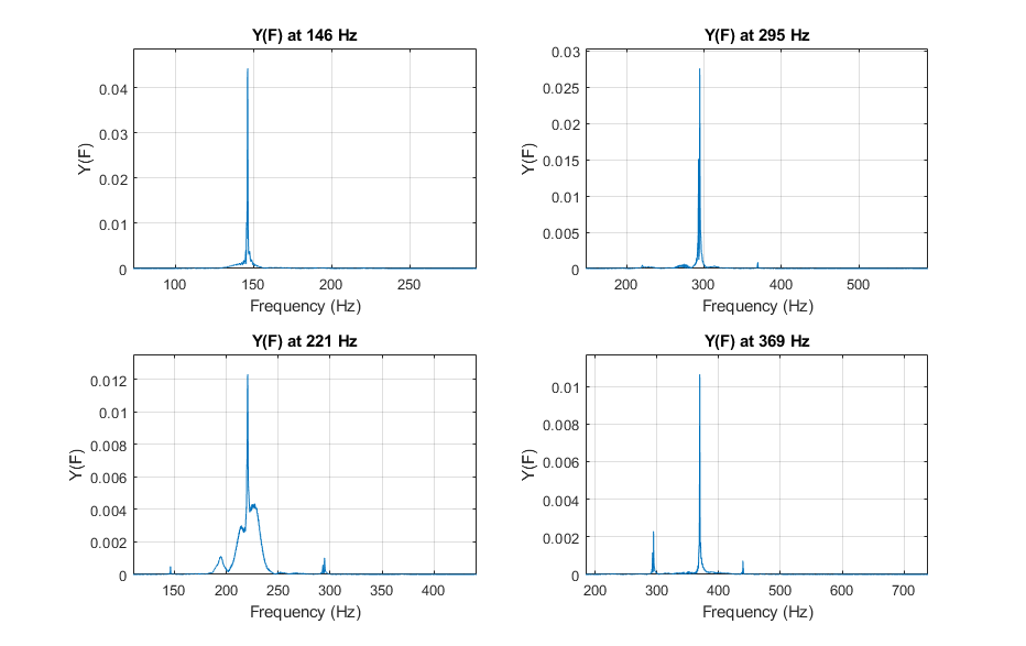

Design Specifications

With the current parameters of a 7th order Chebyshev low pass and high pass filter in series, with center frequencies being 5% above and below the peak frequency respectively, produces an output with each peak being within 3.75% of each other. Scaling was achieved by taking each peak amplitude, finding the median between the highest and lowest amplitude, then generating a factor to make each peak meet the median amplitude. The factors were then multiplied to the frequency domain signal of each filtered isolated peak, and recombined by summing them together. After summation, the peaks of the signal are within 10% of each other. In the following figures a comparison of the original and processed frequency domain signal is shown.

Below shows a comparison between the original signals DFT (left) and the processed signals DFT (right).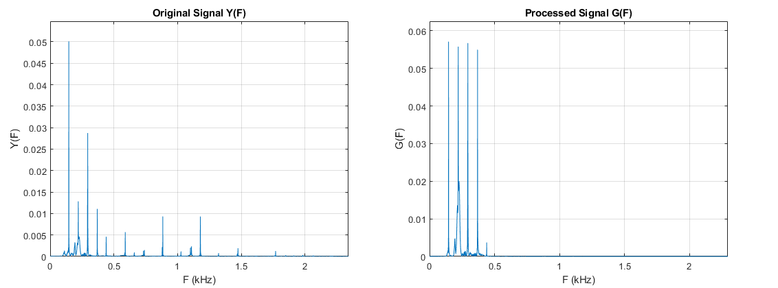

Results

After the process of filtering and equalizing, the processed frequency domain signal was passed through an inverse discrete fourier transform, then normalized to unity. Adjusting parameters greatly affects how the processed signal sounds, and with the current parameters the processed audio signal has a compressed sound to it with a ring you would find in sinusoidal signals without many harmonics. The figures below show a comparison between the original time domain signal and the processed time domain signal.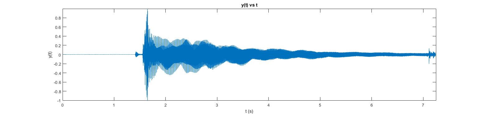

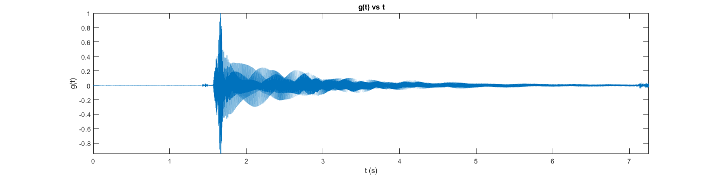
Between the two plots, the compression is visible. This is expected as in the filtering process, most frequencies are being filtered out.

The resulting audio is as follows:

Remarks

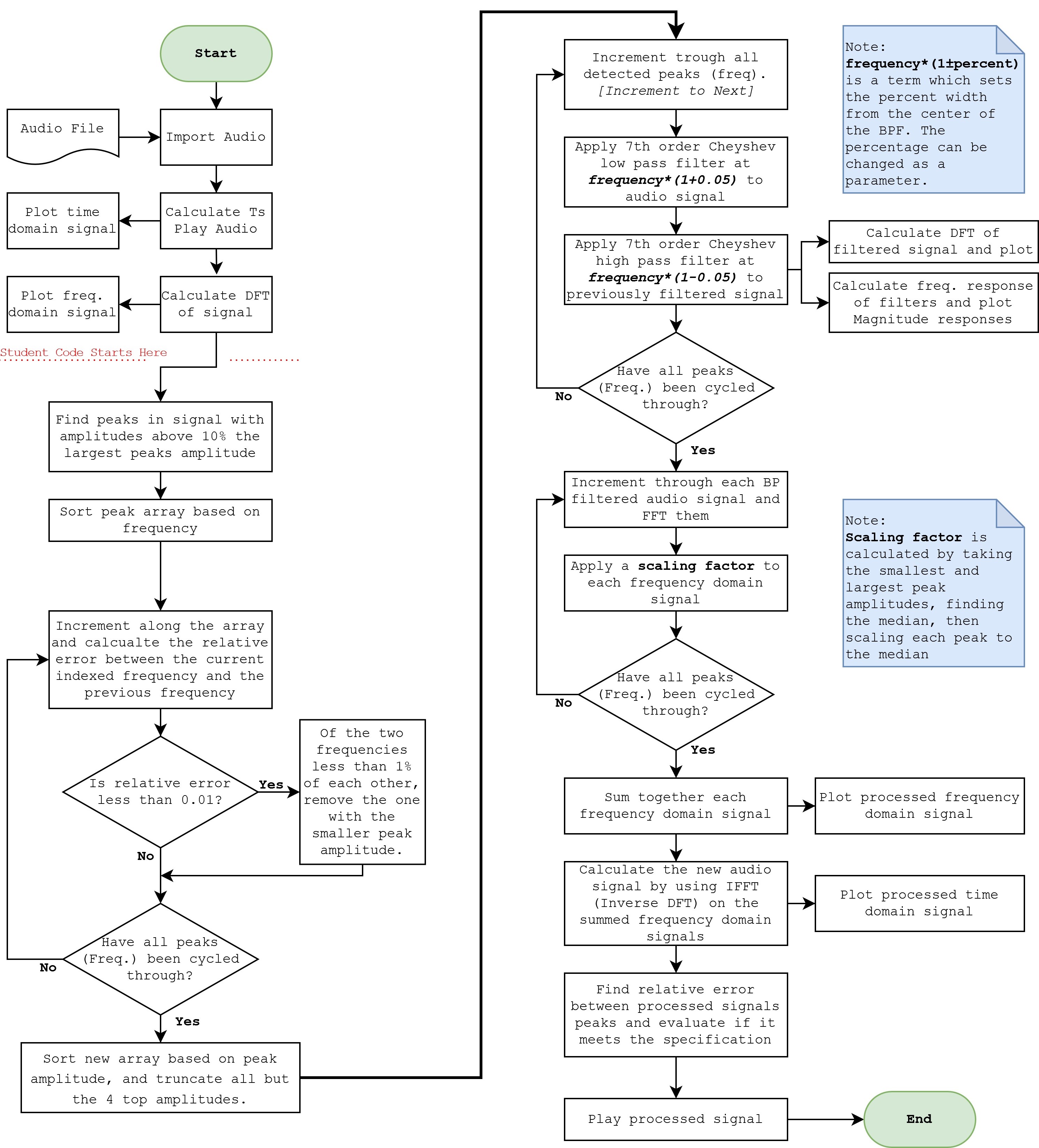
Below is a flowchart of the DSP MATLAB program.