For my antennas course (ENGR 473) in my 4th year of undergraduate studies, the class was given a final project. In this project students were tasked with designing a specific antenna within Cadence's AWR Microwave Office's AXIEM software (I will refer to it as AWR AXIEM, or AXIEM). Students were given a list of antennas they could choose from, such as Yagi-Uda, Bow-tie, Fractal, Helical, etc.

Around the middle of the school term, I was in the process of designing a doublet antenna in the backyard for my HF radio. After a discussion with the professor, he offered I expand on my existing 40m doublet for the project.

The project itself was to hold a presentation educating the class on the history and applications of the antenna, and showing the AWR AXIEM simulation results. In this project writeup I will cover both the process I took of building this antenna and some simulation results.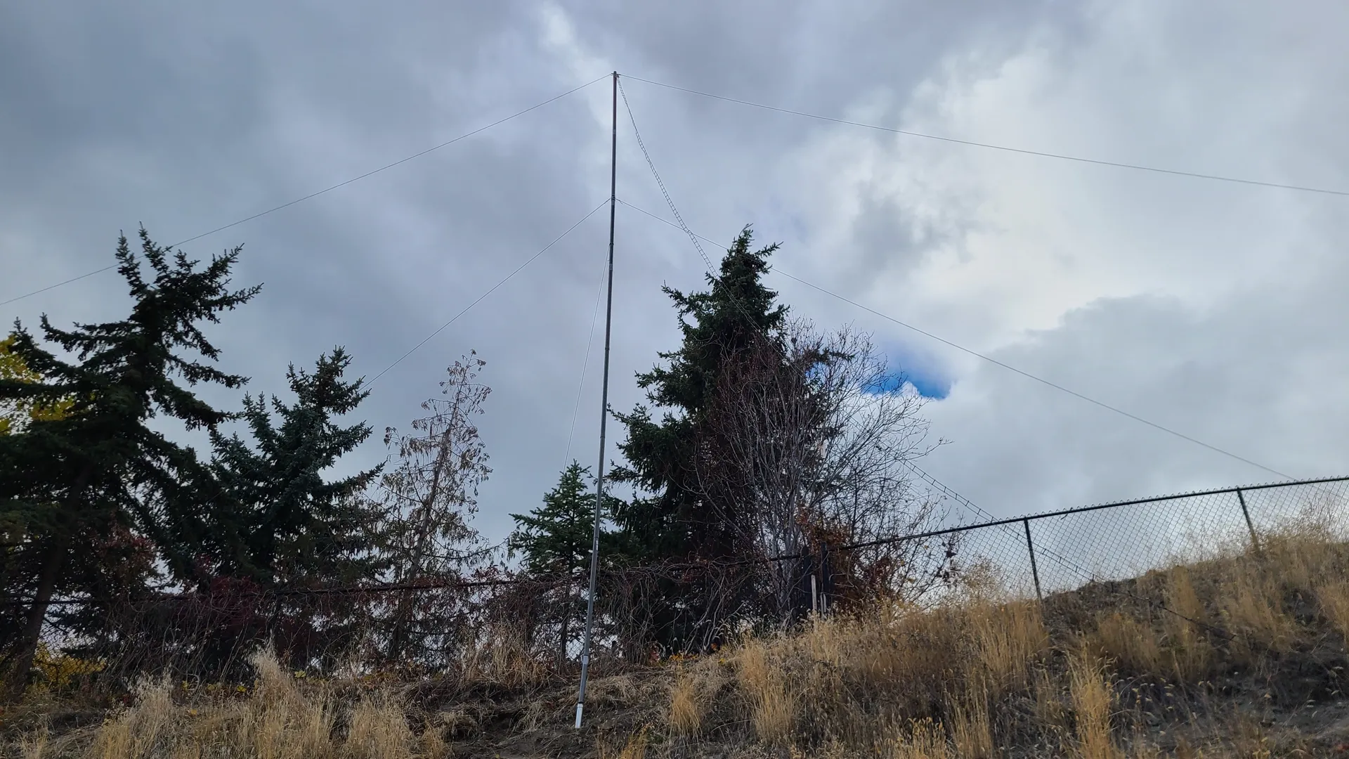

Doublet Antenna

A doublet is a common variant of the standard dipole antenna, but with a few key differences. Most notably, a doublet is a non-resonant dipole that uses a balanced feedline (typically a 300 Ω, 450 Ω, or 600 Ω two-wire "ladder" line). While a standard resonant dipole has an impedance of 73 + j42.5 Ω and easily matches a 50 Ω system with a 1:1 current balun, a doublet's feedline impedance varies wildly depending on the frequency. Because of this, it requires an Antenna Tuning Unit (ATU) to achieve a proper match.

Why use a doublet? It is an incredibly efficient multi-band antenna. Its main draw is the ability to tune across several different frequency bands while maintaining high performance.

What does "non-resonant" mean? In this context, it means the antenna isn't operating at a natural 50 Ω match. The elements are intentionally cut to lengths that do not match the standard wavelength fractions (like λ/2, λ/4, or λ/8) of the frequencies being used.

Note: when referring to λ, it is the wavelength of the lowest operating frequency.

Operation

Because doublets are non-resonant, the VSWR on the elements and balanced feedline can reach 10:1 or higher. If you were to use conventional coaxial cable, cable loss would cause these standing waves to dissipate rather than fully radiate. A two-wire feedline solves this problem: it allows the standing waves to reflect back and forth between the elements and the ATU with very little loss, ensuring most of the energy is radiated.

This balanced feedline also acts as an impedance transformer, a detail that influences how a doublet may be built. By intentionally balancing the lengths of the elements and the feedline, the antenna can be targeted for specific amateur radio bands (most noteably, the 80m/75m, 60m, 40m, 30m, 20m, 17m, 15m, 12m, and 10m bands).

Another approach is to cut the elements to resonate on the lowest desired frequency, while relying on the ATU to tune it for higher bands. For the antenna I built and simulated, I used an element length of 10.7m (approx. 44 feet) to establish a minimum operating frequency of 7 MHz for the 40m band.

Building the Doublet

The antenna was built as affordably as possible. The materials I used to make the antenna were as follows:

• 6x Fiberglass Military tent poles (OD of 2.75-inch) that I found for CA$5 each at Princess Auto.
• A lot of 16 AWG hookup wire that I pulled from a spool I already have.
• 3D printed components, some crimp connectors, and a small fiberglass panel.

Constructing the feedline

Being budget oriented, I decided to construct the feedline myself. To do this, I first calculated the spacing I would need to acieve a 450 Ω characteristic impedance. Using an online two-wire transmission line calculator I determined the best wire spacing to be 28 mm center-to-center. Taking into account the velocity factor of the hookup wire and its PVC insulation, the impedance was likely not exactly 450 Ω, but close.

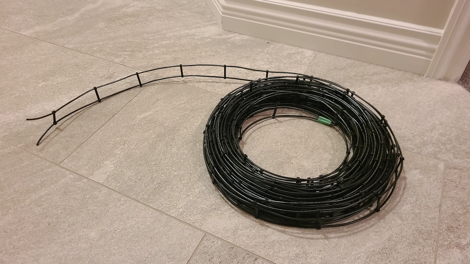
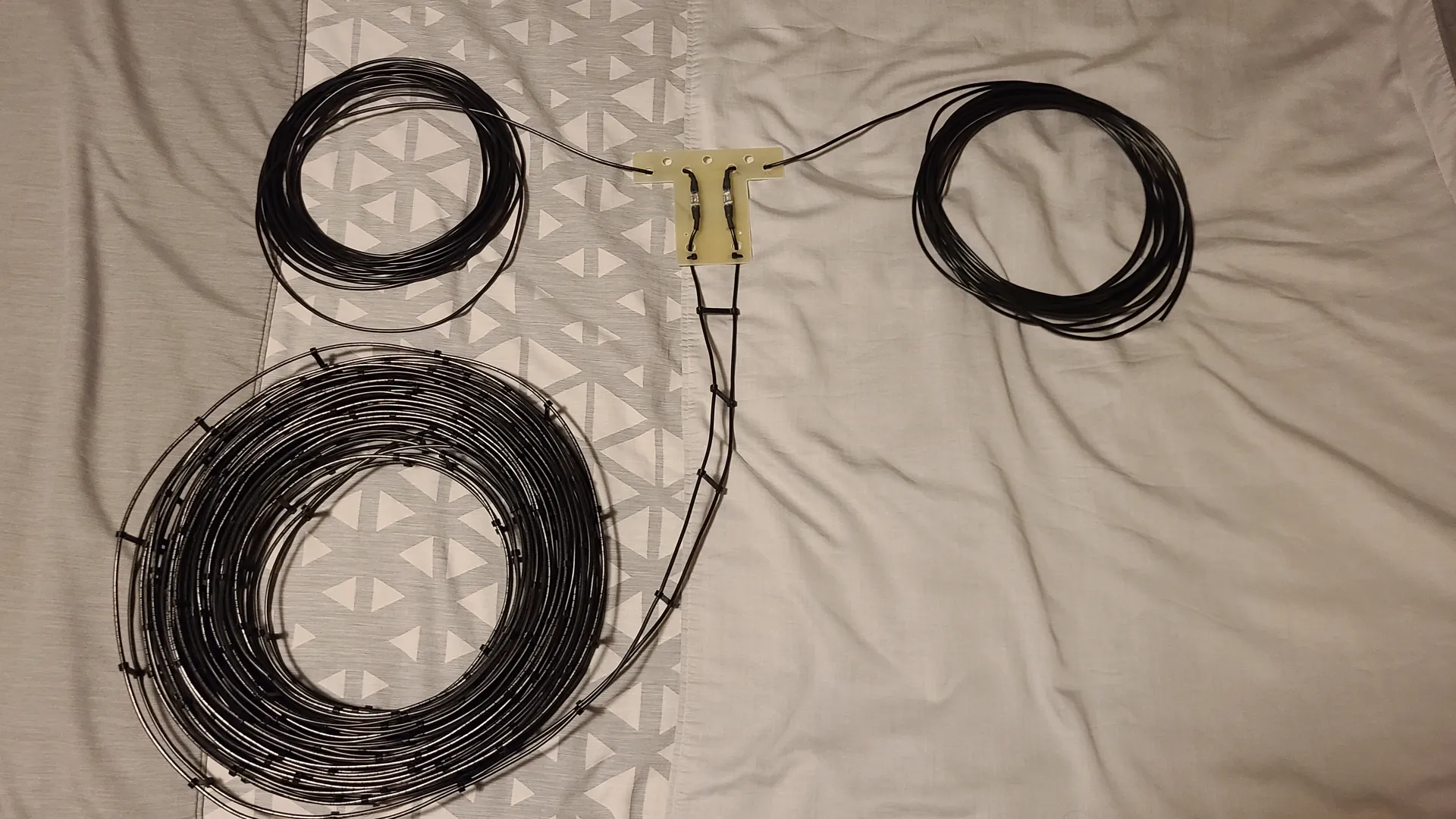
I designed and 3D printed some spacers that snap onto the wire out of PETG plastic. By placing spacers every 5 to 6 inches along the wires I created the feedline.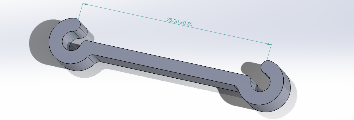

The final feedline was very consistent in its construction and looked the part.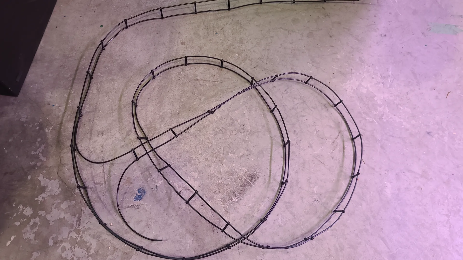

Measuring the elements

The length of each element was cut to 10.7m. This length produces a resonance on the 40m band like a regular dipole antenna, but the doublet configuration allows it to be tunable to multiple bands.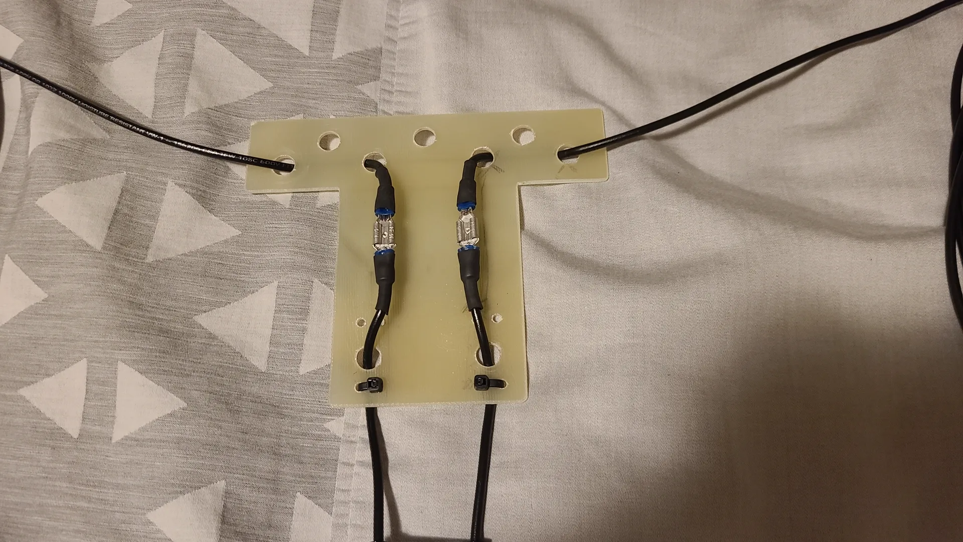

Erecting the Antenna

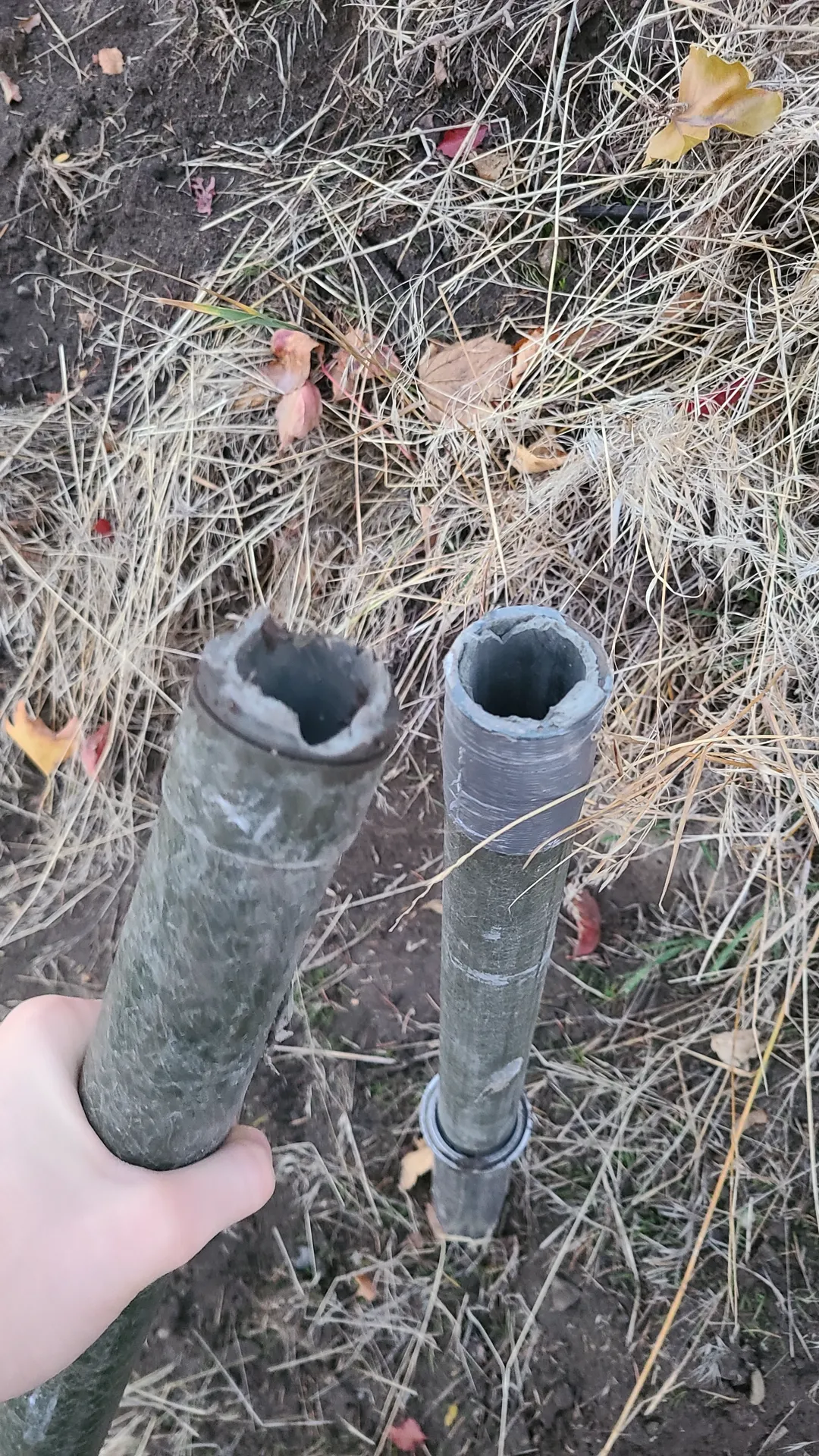
With everything measured and cut, the components were ready to be assembled. I constructed the antenna on the hill behind my house, mounting the fiberglass poles inside a secure steel pipe that I had set into concrete.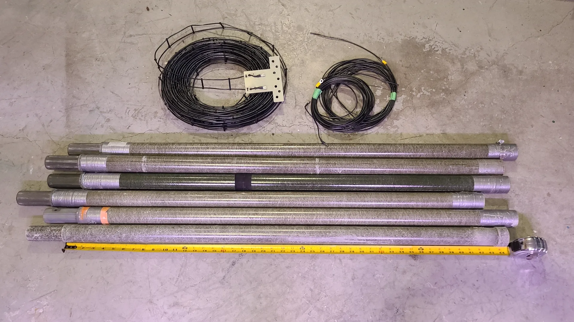

The antenna used 44.25-inch fiberglass military tent poles for its mast. I initially used 8 poles to achieve a height of 10m, but it snapped after an exceptionally windy day. Because of this, I shortened the mast to 6 poles, leaving me with a height of 7.8m. This simply meant the antenna had a higher take-off angle, making it better optimized for NVIS operation.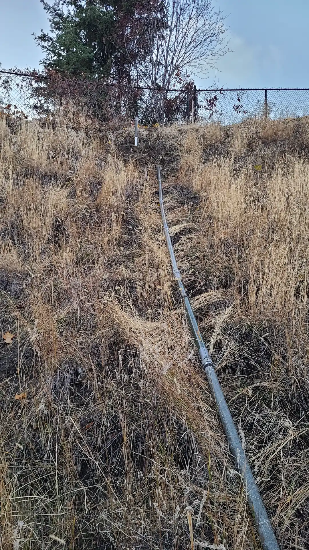

After shortening the mast and optimizing my guy-line placement, the antenna stands strong.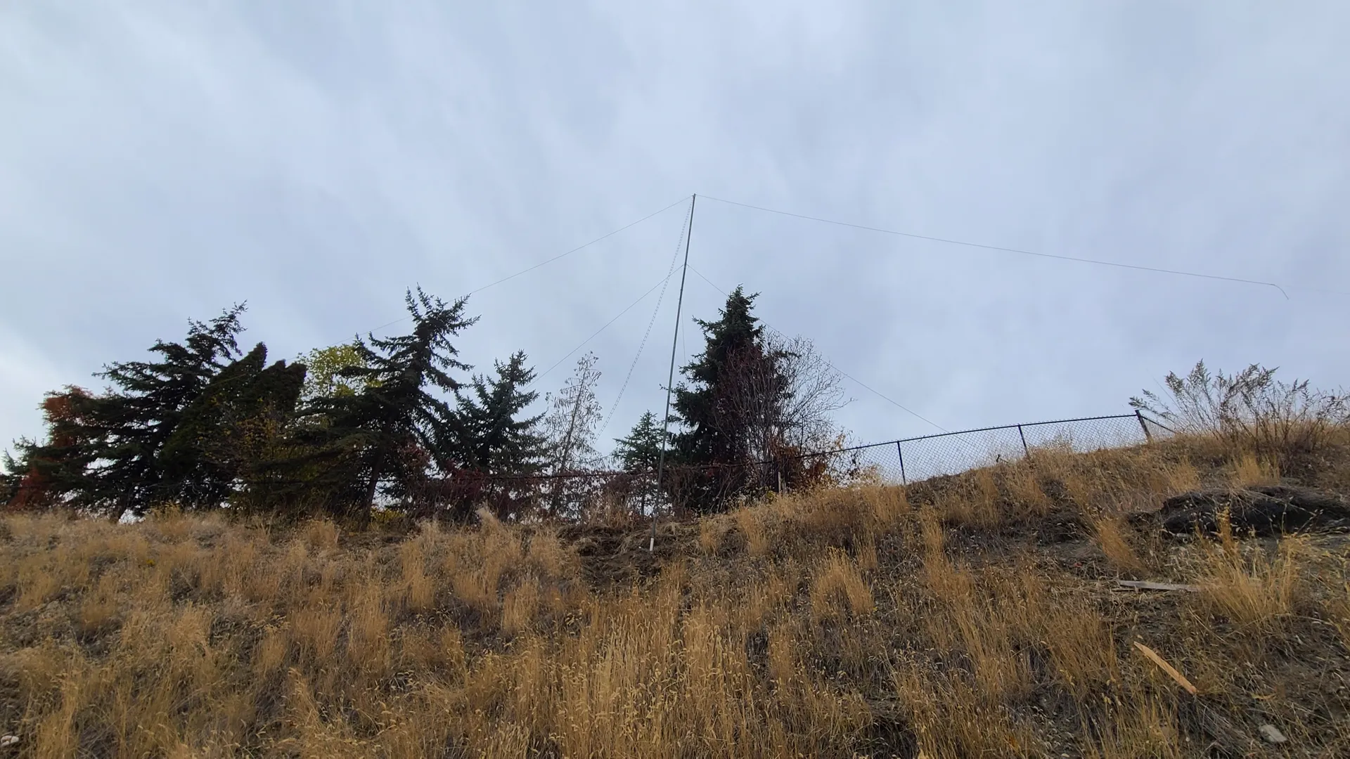

Measurements

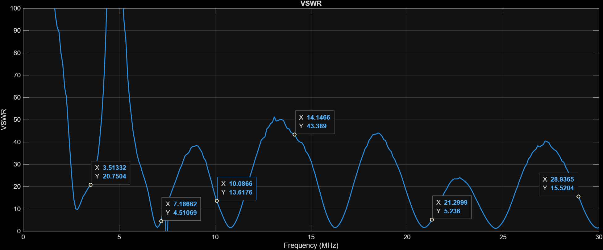
To analyze the antenna's impedance over the 1–30 MHz HF frequency range, I used a 1:1 current balun and a NanoVNA to capture the S11 parameters. I then converted the S11 parameters to a Z11 plot and VSWR plot.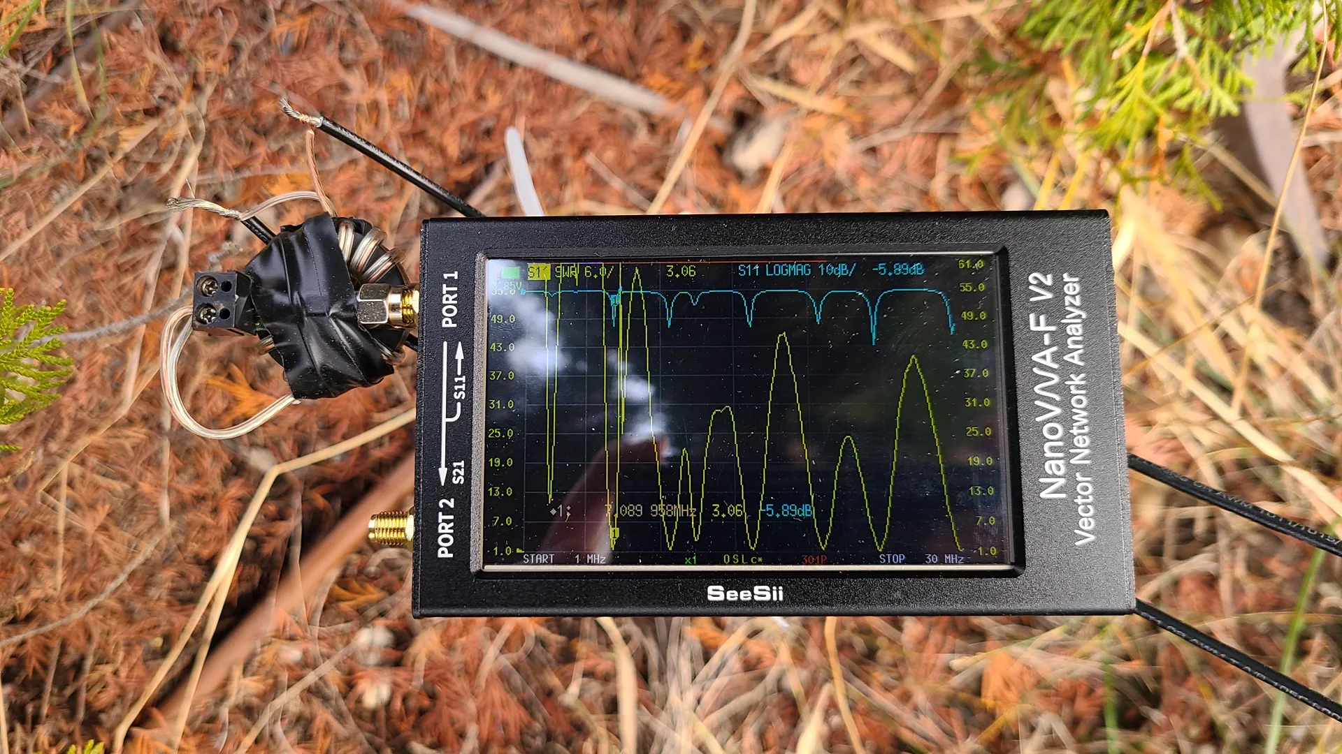

I placed markers on the 80m, 40m, 30m, 20m, 15m, and 10m bands. The resulting impedance at each point will be fed into the ATU via either a 1:1 or 4:1 balun to bring it within a matchable range for a 50 Ω system.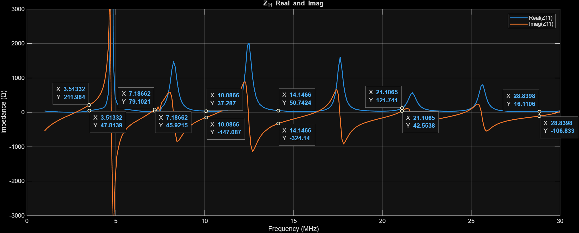

Simulating the Doublet

The doublet was simulated in AWR AXIEM, however due to constraints in the software, I had to scale the antenna and thus its frequency of operation. I scaled the frequency by 100 (and lengths scaled by 0.01). The simulations were run from 500 MHz to 3000 MHz.

I simulated different parameters of the antenna:

• Total feedline length
• Height off ground
• Different earth conductivities

Feedline Length

Since the feedline acts as an impedance transformer, certain configurations can create extreme impedances that are challenging for an ATU to handle. Specifically, it is best to avoid a feedline length that is an integer multiple of λ/2, or any combination where the feedline's electrical length plus one antenna element equals an odd multiple of λ/8 (such as λ/4 + λ/8 = 3λ/8).

The simulation evaluated the resulting impedances for three different feedline lengths: 107.1 mm, 160.7 mm, and 190 mm. The 190 mm feedline yielded the best results, as its non-multiple length provided the most matchable impedances.

Antenna Height

Because the ground mirrors the currents in a horizontally oriented dipole or doublet, the ground plays an integral part in the far-field radiation pattern of the antenna. The best performance is acheived by keeping the antenna λ/2 from the ground or higher. When the antenna elements are less than λ/2 off the ground, the mirrored currents in the ground will act against the antennas currents providing destructive interference. This interference pushes the take-off angle upwards, making the antenna radiate towards the sky rather than the horizon. Having the antenna less than λ/2 or even λ/4 is the principle behind near vertical incidence skywave (NVIS) operation.

The resulting radiation patterns show that as the height off the ground decreases, the main radiating lobe of the lowest frequency is directed further upwards.

Ground Conductivity

Because the ground interacts with the antenna's radiation pattern, I simulated the effect of different earth conductivities based on One-dimensional Layered Earth Models provided by the canadian geological survey.

Presentation Document

The full slide deck can be found in PDF format here: Presentation Slides.